Krylov processes

Krylov processes are the foundation of Krylov methods, they generate bases of Krylov subspaces.

Notation

Define $V_k := \begin{bmatrix} v_1 & \ldots & v_k \end{bmatrix} \enspace$ and $\enspace U_k := \begin{bmatrix} u_1 & \ldots & u_k \end{bmatrix}$.

For a matrix $C \in \mathbb{C}^{n \times n}$ and a vector $t \in \mathbb{C}^{n}$, the $k$-th Krylov subspace generated by $C$ and $t$ is

\[\mathcal{K}_k(C, t) := \left\{\sum_{i=0}^{k-1} \omega_i C^i t \, \middle \vert \, \omega_i \in \mathbb{C},~0 \le i \le k-1 \right\}.\]

For matrices $C \in \mathbb{C}^{n \times n} \enspace$ and $\enspace T \in \mathbb{C}^{n \times p}$, the $k$-th block Krylov subspace generated by $C$ and $T$ is

\[\mathcal{K}_k^{\square}(C, T) := \left\{\sum_{i=0}^{k-1} C^i T \, \Omega_i \, \middle \vert \, \Omega_i \in \mathbb{C}^{p \times p},~0 \le i \le k-1 \right\}.\]

Hermitian Lanczos

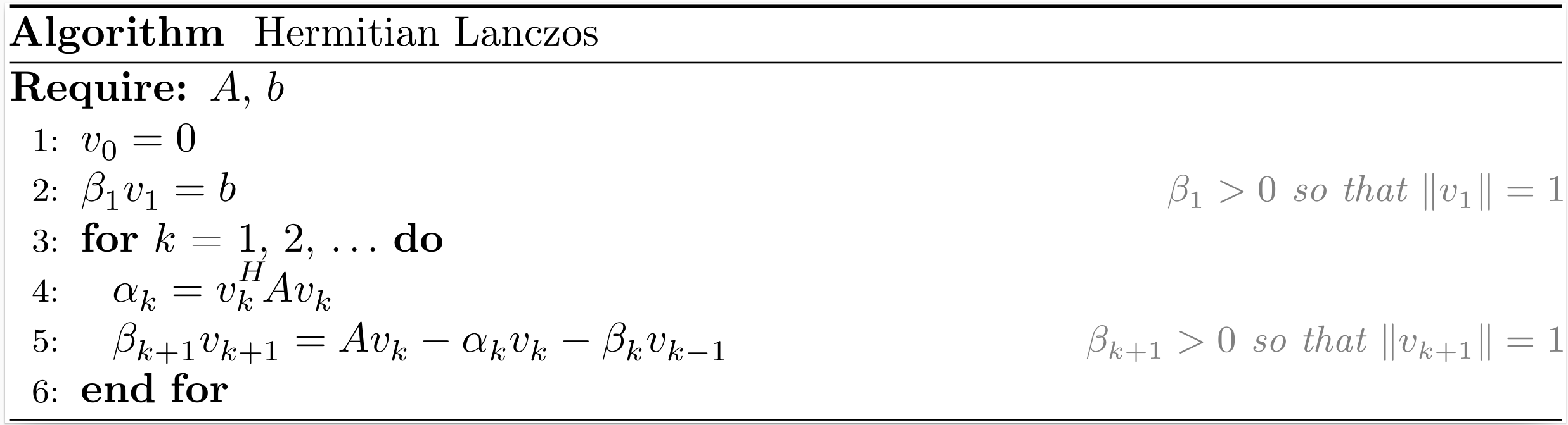
After $k$ iterations of the Hermitian Lanczos process, the situation may be summarized as

\[\begin{align*} A V_k &= V_k T_k + \beta_{k+1,k} v_{k+1} e_k^T = V_{k+1} T_{k+1,k}, \\ V_k^H V_k &= I_k, \end{align*}\]

where $V_k$ is an orthonormal basis of the Krylov subspace $\mathcal{K}_k (A,b)$,

\[T_k = \begin{bmatrix} \alpha_1 & \beta_2 & & \\ \beta_2 & \alpha_2 & \ddots & \\ & \ddots & \ddots & \beta_k \\ & & \beta_k & \alpha_k \end{bmatrix} , \qquad T_{k+1,k} = \begin{bmatrix} T_{k} \\ \beta_{k+1} e_{k}^T \end{bmatrix}.\]

Note that $T_{k+1,k}$ is a real tridiagonal matrix even if $A$ is a complex matrix.

The function hermitian_lanczos returns $V_{k+1}$ and $T_{k+1,k}$.

Related methods: SYMMLQ, CG, CR, MINRES, MINRES-QLP, CGLS, CRLS, CGNE, CRMR, CG-LANCZOS and CG-LANCZOS-SHIFT.

V, T = hermitian_lanczos(A, b, k)

Non-Hermitian Lanczos

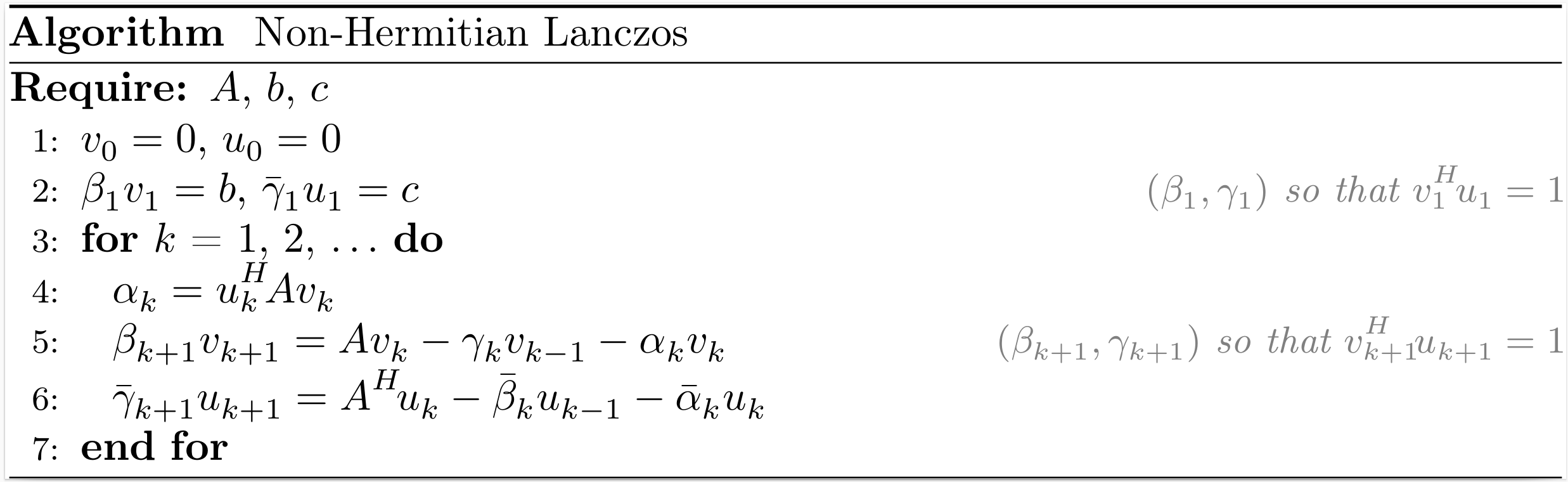
After $k$ iterations of the non-Hermitian Lanczos process (also named the Lanczos biorthogonalization process), the situation may be summarized as

\[\begin{align*} A V_k &= V_k T_k + \beta_{k+1} v_{k+1} e_k^T = V_{k+1} T_{k+1,k}, \\ B U_k &= U_k T_k^H + \bar{\gamma}_{k+1} u_{k+1} e_k^T = U_{k+1} T_{k,k+1}^H, \\ V_k^H U_k &= U_k^H V_k = I_k, \end{align*}\]

where $V_k$ and $U_k$ are bases of the Krylov subspaces $\mathcal{K}_k (A,b)$ and $\mathcal{K}_k (A^H,c)$, respectively,

\[T_k = \begin{bmatrix} \alpha_1 & \gamma_2 & & \\ \beta_2 & \alpha_2 & \ddots & \\ & \ddots & \ddots & \gamma_k \\ & & \beta_k & \alpha_k \end{bmatrix} , \qquad T_{k+1,k} = \begin{bmatrix} T_{k} \\ \beta_{k+1} e_{k}^T \end{bmatrix} , \qquad T_{k,k+1} = \begin{bmatrix} T_{k} & \gamma_{k+1} e_k \end{bmatrix}.\]

The function nonhermitian_lanczos returns $V_{k+1}$, $T_{k+1,k}$, $U_{k+1}$ and $T_{k,k+1}^H$.

Related methods: BiLQ, QMR, BiLQR, CGS and BICGSTAB.

V, T, U, Tᴴ = nonhermitian_lanczos(A, b, c, k)

Arnoldi

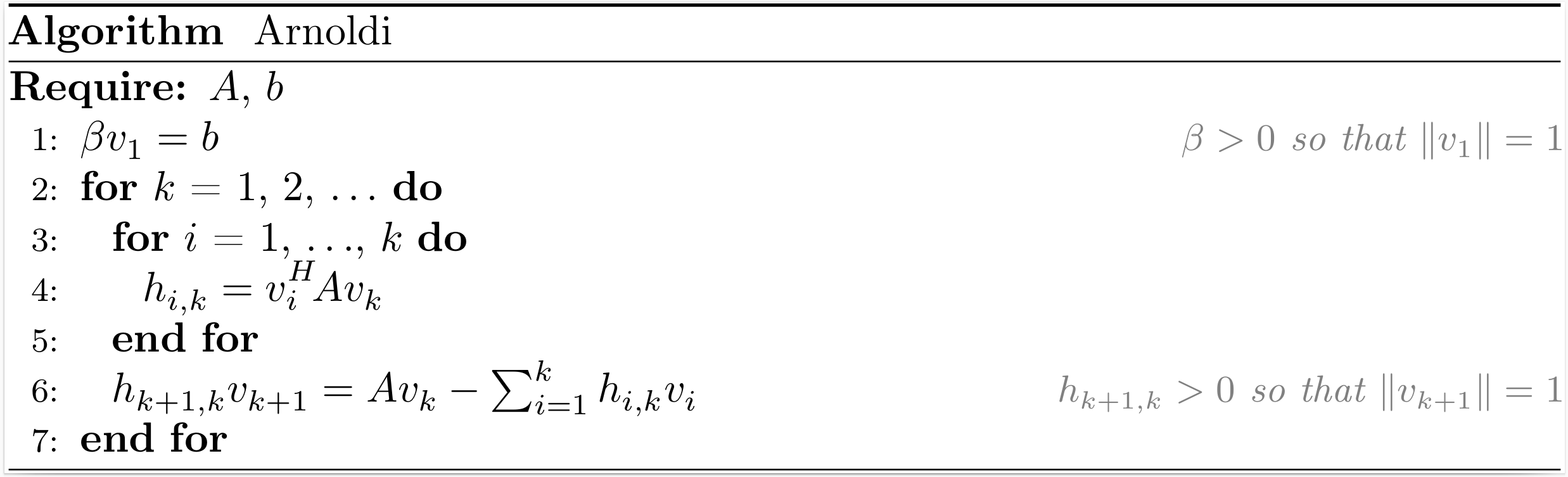
After $k$ iterations of the Arnoldi process, the situation may be summarized as

\[\begin{align*} A V_k &= V_k H_k + h_{k+1,k} v_{k+1} e_k^T = V_{k+1} H_{k+1,k}, \\ V_k^H V_k &= I_k, \end{align*}\]

where $V_k$ is an orthonormal basis of the Krylov subspace $\mathcal{K}_k (A,b)$,

\[H_k = \begin{bmatrix} h_{1,1}~ & h_{1,2}~ & \ldots & h_{1,k} \\ h_{2,1}~ & \ddots~ & \ddots & \vdots \\ & \ddots~ & \ddots & h_{k-1,k} \\ & & h_{k,k-1} & h_{k,k} \end{bmatrix} , \qquad H_{k+1,k} = \begin{bmatrix} H_{k} \\ h_{k+1,k} e_{k}^T \end{bmatrix}.\]

The function arnoldi returns $V_{k+1}$ and $H_{k+1,k}$.

Related methods: DIOM, FOM, DQGMRES and GMRES.

V, H = arnoldi(A, b, k)

Golub-Kahan

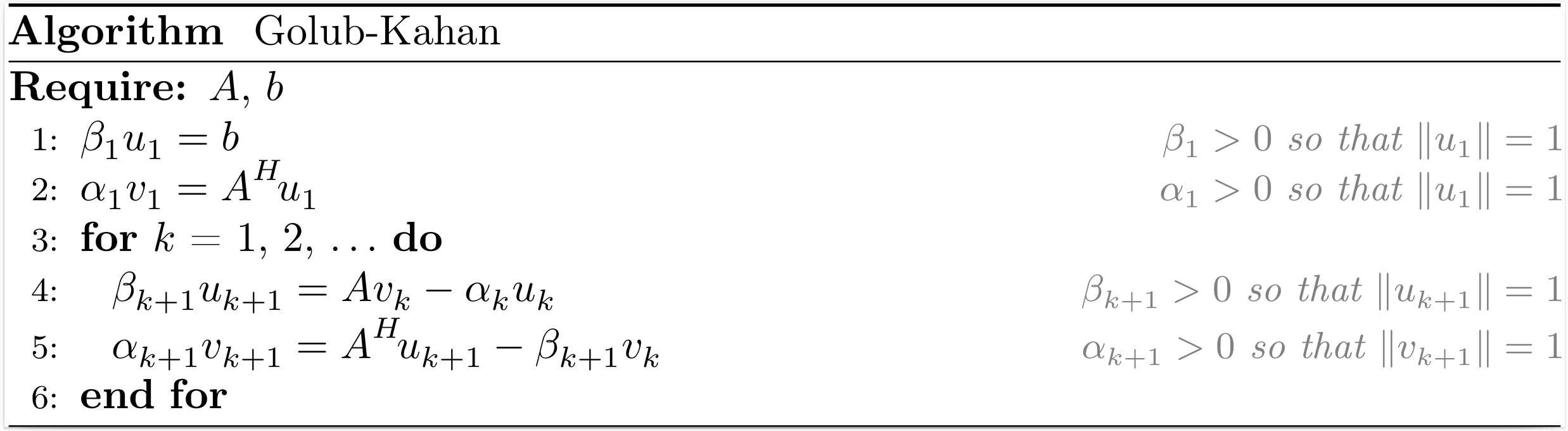
After $k$ iterations of the Golub-Kahan bidiagonalization process, the situation may be summarized as

\[\begin{align*} A V_k &= U_{k+1} B_k, \\ A^H U_{k+1} &= V_k B_k^H + \alpha_{k+1} v_{k+1} e_{k+1}^T = V_{k+1} L_{k+1}^H, \\ V_k^H V_k &= U_k^H U_k = I_k, \end{align*}\]

where $V_k$ and $U_k$ are bases of the Krylov subspaces $\mathcal{K}_k (A^HA,A^Hb)$ and $\mathcal{K}_k (AA^H,b)$, respectively,

\[L_k = \begin{bmatrix} \alpha_1 & & & \\ \beta_2 & \alpha_2 & & \\ & \ddots & \ddots & \\ & & \beta_k & \alpha_k \end{bmatrix} , \qquad B_k = \begin{bmatrix} \alpha_1 & & & \\ \beta_2 & \alpha_2 & & \\ & \ddots & \ddots & \\ & & \beta_k & \alpha_k \\ & & & \beta_{k+1} \\ \end{bmatrix} = \begin{bmatrix} L_{k} \\ \beta_{k+1} e_{k}^T \end{bmatrix}.\]

Note that $L_k$ is a real bidiagonal matrix even if $A$ is a complex matrix.

The function golub_kahan returns $V_{k+1}$, $U_{k+1}$ and $L_{k+1}$.

Related methods: LNLQ, CRAIG, CRAIGMR, LSLQ, LSQR and LSMR.

V, U, L = golub_kahan(A, b, k)

Saunders-Simon-Yip

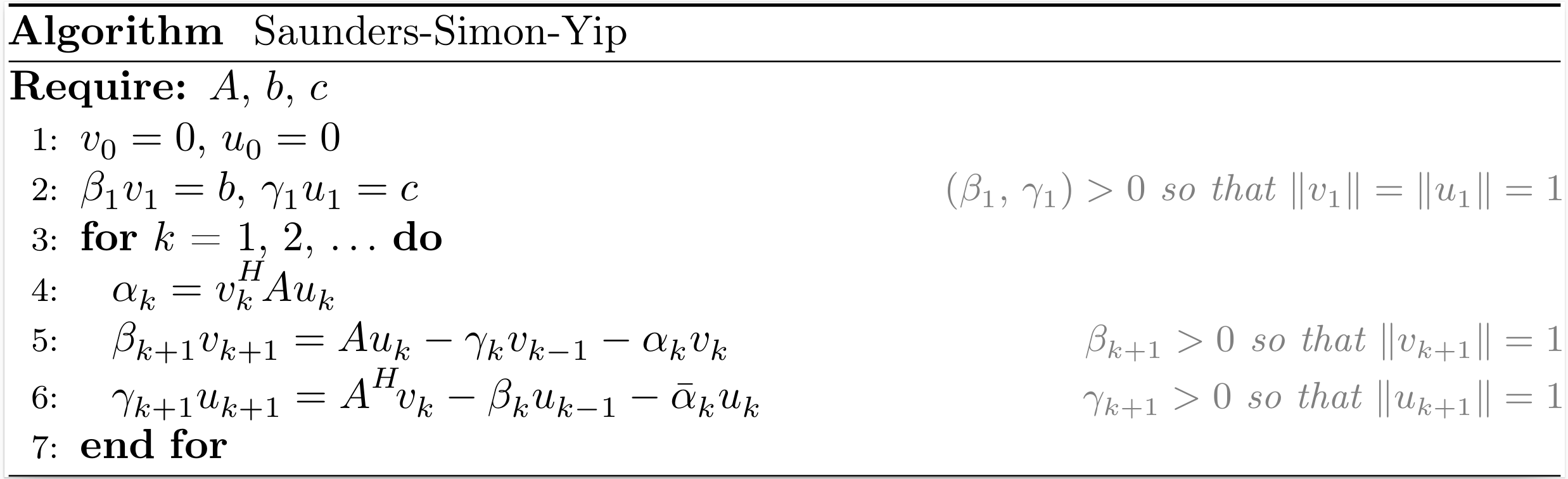
After $k$ iterations of the Saunders-Simon-Yip process (also named the orthogonal tridiagonalization process), the situation may be summarized as

\[\begin{align*} A U_k &= V_k T_k + \beta_{k+1} v_{k+1} e_k^T = V_{k+1} T_{k+1,k}, \\ B V_k &= U_k T_k^H + \gamma_{k+1} u_{k+1} e_k^T = U_{k+1} T_{k,k+1}^H, \\ V_k^H V_k &= U_k^H U_k = I_k, \end{align*}\]

where $\begin{bmatrix} V_k & 0 \\ 0 & U_k \end{bmatrix}$ is an orthonormal basis of the block Krylov subspace $\mathcal{K}^{\square}_k \left(\begin{bmatrix} 0 & A \\ A^H & 0 \end{bmatrix}, \begin{bmatrix} b & 0 \\ 0 & c \end{bmatrix}\right)$,

\[T_k = \begin{bmatrix} \alpha_1 & \gamma_2 & & \\ \beta_2 & \alpha_2 & \ddots & \\ & \ddots & \ddots & \gamma_k \\ & & \beta_k & \alpha_k \end{bmatrix} , \qquad T_{k+1,k} = \begin{bmatrix} T_{k} \\ \beta_{k+1} e_{k}^T \end{bmatrix} , \qquad T_{k,k+1} = \begin{bmatrix} T_{k} & \gamma_{k+1} e_{k} \end{bmatrix}.\]

The function saunders_simon_yip returns $V_{k+1}$, $T_{k+1,k}$, $U_{k+1}$ and $T_{k,k+1}^H$.

Related methods: USYMLQ, USYMQR, TriLQR, TriCG and TriMR.

V, T, U, Tᴴ = saunders_simon_yip(A, b, c, k)

Montoison-Orban

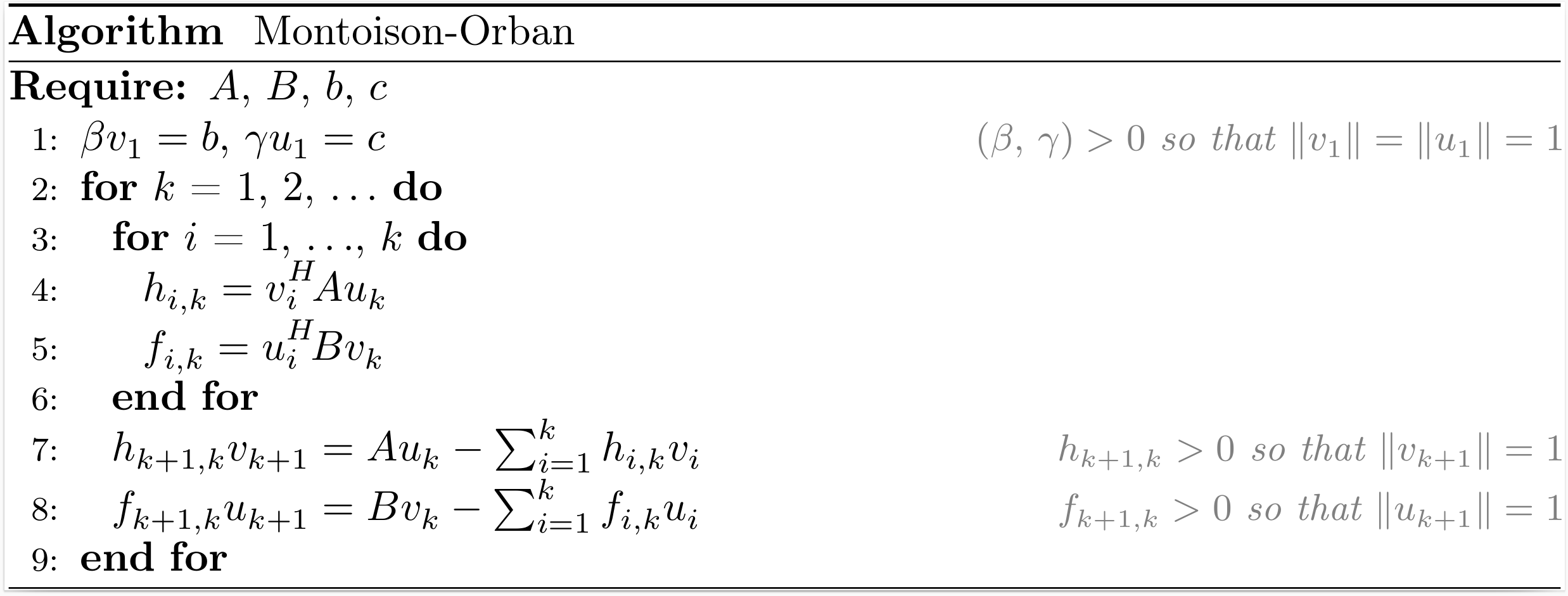
After $k$ iterations of the Montoison-Orban process (also named the orthogonal Hessenberg reduction process), the situation may be summarized as

\[\begin{align*} A U_k &= V_k H_k + h_{k+1,k} v_{k+1} e_k^T = V_{k+1} H_{k+1,k}, \\ B V_k &= U_k F_k + f_{k+1,k} u_{k+1} e_k^T = U_{k+1} F_{k+1,k}, \\ V_k^H V_k &= U_k^H U_k = I_k, \end{align*}\]

where $\begin{bmatrix} V_k & 0 \\ 0 & U_k \end{bmatrix}$ is an orthonormal basis of the block Krylov subspace $\mathcal{K}^{\square}_k \left(\begin{bmatrix} 0 & A \\ B & 0 \end{bmatrix}, \begin{bmatrix} b & 0 \\ 0 & c \end{bmatrix}\right)$,

\[H_k = \begin{bmatrix} h_{1,1}~ & h_{1,2}~ & \ldots & h_{1,k} \\ h_{2,1}~ & \ddots~ & \ddots & \vdots \\ & \ddots~ & \ddots & h_{k-1,k} \\ & & h_{k,k-1} & h_{k,k} \end{bmatrix} , \qquad F_k = \begin{bmatrix} f_{1,1}~ & f_{1,2}~ & \ldots & f_{1,k} \\ f_{2,1}~ & \ddots~ & \ddots & \vdots \\ & \ddots~ & \ddots & f_{k-1,k} \\ & & f_{k,k-1} & f_{k,k} \end{bmatrix},\]

\[H_{k+1,k} = \begin{bmatrix} H_{k} \\ h_{k+1,k} e_{k}^T \end{bmatrix} , \qquad F_{k+1,k} = \begin{bmatrix} F_{k} \\ f_{k+1,k} e_{k}^T \end{bmatrix}.\]

The function montoison_orban returns $V_{k+1}$, $H_{k+1,k}$, $U_{k+1}$ and $F_{k+1,k}$.

Related methods: GPMR.

V, H, U, F = montoison_orban(A, B, b, c, k)