by Abel S. Siqueira and João Okimoto


In this tutorial you will learn what is a JSO-compliant solver, how to create one, and how to benchmark it against some other solver.
A JSO-compliant solver is a solver whose
That means that you can devise your solver based on a single API that will work with many different problems. Furthermore, since the output type is known, we can provide tools to compare different solvers.
To illustrate the procedure for creating a solver with the JSO API, we'll implement a Line-Search Modified Newton solver for the problem
\[ \min_x \ f(x) \]
The method consists of following the direction \(d_k\) that solves
\[ \nabla^2 f(x_k) d_k = -\nabla f(x_k) \]
This is only reasonable if the system can be solved and \(d_k\) is a descent direction. A sufficient condition for that is that \(\nabla^2 f(x_k)\) is positive definite, which is equivalent to saying that it has a Cholesky decomposition.
Since this will not be true in general, the modified Newton method consists of computing \(\rho_k \geq 0\) such that \(\nabla^2 f(x_k) + \rho_k I\) is positive definite. One way to find such a \(\rho_k\) is given below
1. Start with ρ from the last iteration
2. Try to compute the Cholesky factor of ∇²f(x) + ρI
3. If not successful, increase ρ to either 1e-8 or 10ρ, whichever is largest, and return to step 2
4. Otherwise, continue the algorithm
Next, for the line-search part, we use backtracking and ask that the Armijo condition be satisfied, that is find the smallest \(p \in \mathbb{N}\) such that \(t = σ^p\) satisfies
\[ f(x_k + td_k) < f(x_k) + \alpha t g_k^T d_k, \]
for \(\alpha \in (0,1)\), called the Armijo parameter.
Let's define a test problem to verify that our method is working, and let's use a classic one: Rosenbrock's function[1]
\[ \min_x \ (x_1 - 1)^2 + 4 (x_2 - x_1^2)^2, \]
starting from point [-1.2; 1.0].
using Plots
gr(size=(600,300))
contour(-2:0.02:2, -0.5:0.02:1.5, (x,y) -> (x - 1)^2 + 4 * (y - x^2)^2, levels=(0:0.2:10).^2)
title!("Contour plot of objective")
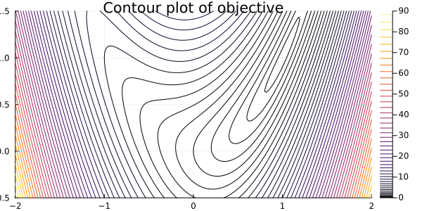
Notice that the solution of the problem, i.e., the point at which the function is minimum, is \(x = (1,1)^T\). This can be estimated by the plot and verified by noticing that \(f(1,1) = 0\) and \(f(x) > 0\) for any other point.
To write this problem as a NLPModel, we have a few options, but for now let's consider the simplest one: ADNLPModels. ADNLPModels has a simple interface and it computes the derivatives using automatic differentiation from other packages.
using ADNLPModels

nlp = ADNLPModel(
  x -> (x[1] - 1)^2 + 4 * (x[2] - x[1]^2)^2, # function
  [-1.2; 1.0] # starting point
)
ADNLPModel - Model with automatic differentiation backend ADModelBackend{
  ForwardDiffADGradient,
  ForwardDiffADHvprod,
  EmptyADbackend,
  EmptyADbackend,
  EmptyADbackend,
  ForwardDiffADHessian,
  EmptyADbackend,
}
  Problem name: Generic
   All variables: ████████████████████ 2      All constraints: ⋅⋅⋅⋅⋅⋅⋅⋅⋅⋅⋅⋅⋅⋅⋅⋅⋅⋅⋅⋅ 0
            free: ████████████████████ 2                 free: ⋅⋅⋅⋅⋅⋅⋅⋅⋅⋅⋅⋅⋅⋅⋅⋅⋅⋅⋅⋅ 0
           lower: ⋅⋅⋅⋅⋅⋅⋅⋅⋅⋅⋅⋅⋅⋅⋅⋅⋅⋅⋅⋅ 0                lower: ⋅⋅⋅⋅⋅⋅⋅⋅⋅⋅⋅⋅⋅⋅⋅⋅⋅⋅⋅⋅ 0
           upper: ⋅⋅⋅⋅⋅⋅⋅⋅⋅⋅⋅⋅⋅⋅⋅⋅⋅⋅⋅⋅ 0                upper: ⋅⋅⋅⋅⋅⋅⋅⋅⋅⋅⋅⋅⋅⋅⋅⋅⋅⋅⋅⋅ 0
         low/upp: ⋅⋅⋅⋅⋅⋅⋅⋅⋅⋅⋅⋅⋅⋅⋅⋅⋅⋅⋅⋅ 0              low/upp: ⋅⋅⋅⋅⋅⋅⋅⋅⋅⋅⋅⋅⋅⋅⋅⋅⋅⋅⋅⋅ 0
           fixed: ⋅⋅⋅⋅⋅⋅⋅⋅⋅⋅⋅⋅⋅⋅⋅⋅⋅⋅⋅⋅ 0                fixed: ⋅⋅⋅⋅⋅⋅⋅⋅⋅⋅⋅⋅⋅⋅⋅⋅⋅⋅⋅⋅ 0
          infeas: ⋅⋅⋅⋅⋅⋅⋅⋅⋅⋅⋅⋅⋅⋅⋅⋅⋅⋅⋅⋅ 0               infeas: ⋅⋅⋅⋅⋅⋅⋅⋅⋅⋅⋅⋅⋅⋅⋅⋅⋅⋅⋅⋅ 0
            nnzh: (  0.00% sparsity)   3               linear: ⋅⋅⋅⋅⋅⋅⋅⋅⋅⋅⋅⋅⋅⋅⋅⋅⋅⋅⋅⋅ 0
                                                    nonlinear: ⋅⋅⋅⋅⋅⋅⋅⋅⋅⋅⋅⋅⋅⋅⋅⋅⋅⋅⋅⋅ 0
                                                         nnzj: (------% sparsity)

  Counters:
             obj: ⋅⋅⋅⋅⋅⋅⋅⋅⋅⋅⋅⋅⋅⋅⋅⋅⋅⋅⋅⋅ 0                 grad: ⋅⋅⋅⋅⋅⋅⋅⋅⋅⋅⋅⋅⋅⋅⋅⋅⋅⋅⋅⋅ 0                 cons: ⋅⋅⋅⋅⋅⋅⋅⋅⋅⋅⋅⋅⋅⋅⋅⋅⋅⋅⋅⋅ 0
        cons_lin: ⋅⋅⋅⋅⋅⋅⋅⋅⋅⋅⋅⋅⋅⋅⋅⋅⋅⋅⋅⋅ 0             cons_nln: ⋅⋅⋅⋅⋅⋅⋅⋅⋅⋅⋅⋅⋅⋅⋅⋅⋅⋅⋅⋅ 0                 jcon: ⋅⋅⋅⋅⋅⋅⋅⋅⋅⋅⋅⋅⋅⋅⋅⋅⋅⋅⋅⋅ 0
           jgrad: ⋅⋅⋅⋅⋅⋅⋅⋅⋅⋅⋅⋅⋅⋅⋅⋅⋅⋅⋅⋅ 0                  jac: ⋅⋅⋅⋅⋅⋅⋅⋅⋅⋅⋅⋅⋅⋅⋅⋅⋅⋅⋅⋅ 0              jac_lin: ⋅⋅⋅⋅⋅⋅⋅⋅⋅⋅⋅⋅⋅⋅⋅⋅⋅⋅⋅⋅ 0
         jac_nln: ⋅⋅⋅⋅⋅⋅⋅⋅⋅⋅⋅⋅⋅⋅⋅⋅⋅⋅⋅⋅ 0                jprod: ⋅⋅⋅⋅⋅⋅⋅⋅⋅⋅⋅⋅⋅⋅⋅⋅⋅⋅⋅⋅ 0            jprod_lin: ⋅⋅⋅⋅⋅⋅⋅⋅⋅⋅⋅⋅⋅⋅⋅⋅⋅⋅⋅⋅ 0
       jprod_nln: ⋅⋅⋅⋅⋅⋅⋅⋅⋅⋅⋅⋅⋅⋅⋅⋅⋅⋅⋅⋅ 0               jtprod: ⋅⋅⋅⋅⋅⋅⋅⋅⋅⋅⋅⋅⋅⋅⋅⋅⋅⋅⋅⋅ 0           jtprod_lin: ⋅⋅⋅⋅⋅⋅⋅⋅⋅⋅⋅⋅⋅⋅⋅⋅⋅⋅⋅⋅ 0
      jtprod_nln: ⋅⋅⋅⋅⋅⋅⋅⋅⋅⋅⋅⋅⋅⋅⋅⋅⋅⋅⋅⋅ 0                 hess: ⋅⋅⋅⋅⋅⋅⋅⋅⋅⋅⋅⋅⋅⋅⋅⋅⋅⋅⋅⋅ 0                hprod: ⋅⋅⋅⋅⋅⋅⋅⋅⋅⋅⋅⋅⋅⋅⋅⋅⋅⋅⋅⋅ 0
           jhess: ⋅⋅⋅⋅⋅⋅⋅⋅⋅⋅⋅⋅⋅⋅⋅⋅⋅⋅⋅⋅ 0               jhprod: ⋅⋅⋅⋅⋅⋅⋅⋅⋅⋅⋅⋅⋅⋅⋅⋅⋅⋅⋅⋅ 0
Now we access the information of the model, and its functions. The information is all stored on nlp.meta, while the functions are defined by NLPModels.
The main information you may want is summarised below
(
  nlp.meta.nvar, # number of variable
  nlp.meta.ncon, # number of constraints
  nlp.meta.lvar, nlp.meta.uvar, # bounds on variables
  nlp.meta.lcon, nlp.meta.ucon, # bounds on constraints
  nlp.meta.x0 # starting point
)
(2, 0, [-Inf, -Inf], [Inf, Inf], Float64[], Float64[], [-1.2, 1.0])
Furthermore, you can use some functions from NLPModels to query whether the problem has bounds, equalities, inequalities, etc.
using NLPModels

unconstrained(nlp)
true
Finally, we can access the objective function, its gradients and Hessian with
x = nlp.meta.x0
obj(nlp, x)
5.614400000000001
grad(nlp, x)
2-element Vector{Float64}:
 -12.847999999999999
  -3.5199999999999996
hess(nlp, x)
2×2 LinearAlgebra.Symmetric{Float64, SparseArrays.SparseMatrixCSC{Float64, Int64}}:
 55.12  19.2
 19.2    8.0
For our basic unconstrained solver that's enough. If you want more functions, check the NLPModels reference guide.
Notice that the Hessian returned from hess has only the lower triangle. That's done, in general, to avoid storing repeated elements. In this dense case, this isn't much helpful, so we can simply use Symmetric to fill the rest.
using LinearAlgebra

Symmetric(hess(nlp, x), :L)
2×2 LinearAlgebra.Symmetric{Float64, SparseArrays.SparseMatrixCSC{Float64, Int64}}:
 55.12  19.2
 19.2    8.0
To compute Cholesky and verify that it succeeds, we use cholesky and issuccess.
B = Symmetric(hess(nlp, x), :L)
factor = cholesky(B, check=false) # check is false to prevent an error from being thrown.
issuccess(factor)
true
B = -Symmetric(hess(nlp, x), :L) # Since the last one is positive definite, this one shouldn't be
factor = cholesky(B, check=false)
issuccess(factor)
false
Therefore the direction computation can be done as
ρ = 0.0 # First iteration

B = Symmetric(hess(nlp, x), :L)
factor = cholesky(B + ρ * I, check=false)
while !issuccess(factor)
  ρ = max(1e-8, 10ρ)
  factor = cholesky(B + ρ * I, check=false)
end
d = factor \ -grad(nlp, x)
2-element Vector{Float64}:
  0.4867256637168144
 -0.7281415929203547
The second part of our method is the step length computation. Let's use α = 1e-2 for our Armijo parameter.
α = 1e-2
t = 1.0
fx = obj(nlp, x)
ft = obj(nlp, x + t * d)
slope = dot(grad(nlp, x), d)
while !(ft ≤ fx + t * slope)
  global t *= 0.5 # global is used because we are outside a function
  ft = obj(nlp, x + t * d)
end
The two snippets above are what define our method. We'll use the first order criteria for stopping the algorithm, that is
\[ \| \nabla f(x_k) \| < \epsilon \]
using SolverCore

function newton(nlp :: AbstractNLPModel)

  x = copy(nlp.meta.x0) # starting point
  α = 1e-2 # Armijo parameter
  ρ = 0.0

  while norm(grad(nlp, x)) > 1e-6

    # Computing the direction
    B = Symmetric(hess(nlp, x), :L)
    factor = cholesky(B + ρ * I, check=false)
    while !issuccess(factor)
      ρ = max(1e-8, 10ρ)
      factor = cholesky(B + ρ * I, check=false)
    end
    d = factor \ -grad(nlp, x)

    # Computing the step length
    t = 1.0
    fx = obj(nlp, x)
    ft = obj(nlp, x + t * d)
    slope = dot(grad(nlp, x), d)
    while !(ft ≤ fx + α * t * slope)
      t *= 0.5
      ft = obj(nlp, x + t * d)
    end

    x += t * d
  end

  status = :first_order

  return GenericExecutionStats(nlp, status=status)

end
newton (generic function with 1 method)
Notice the two conditions for the method to be JSO-compliant:
function newton(nlp :: AbstractNLPModel)
return GenericExecutionStats(status, nlp)
For this structure to be used, a status argument needs to be passed, indicating what's the situation of the solver run. We passed a :first_order value, indicating that a first order solution was found. More about this later.
The NLPModels API provides you with the derivatives, and anything else can reside inside the function, and there is where the magic happens.
Let's run our implementation on the problem we defined before.
output = newton(nlp)

println(output)
Generic Execution stats
  status: first-order stationary
  objective value: Inf
  primal feasibility: 0.0
  dual feasibility: Inf
  solution: [0.0  0.0]
  iterations: -1
  elapsed time: Inf
The GenericExecutionStats structure holds all relevant information. Notice, however, that it doesn't have anything useful in this case. Naturally, we have to return that information as well.
Update your newton function so that the end is something like the following.
function newton(nlp :: AbstractNLPModel)
  # …

  return GenericExecutionStats(nlp, status=status, solution=x, objective=obj(nlp, x))
end
newton (generic function with 1 method)
Now run again
output = newton(nlp)

println(output)
Generic Execution stats
  status: first-order stationary
  objective value: 7.141610295610004e-18
  primal feasibility: 0.0
  dual feasibility: Inf
  solution: [0.9999999973418803  0.9999999945459112]
  iterations: -1
  elapsed time: Inf
That's already better. Now we can access the solution with
output.solution
2-element Vector{Float64}:
 0.9999999973418803
 0.9999999945459112
Although we have an implementation of our method, it has a few shortcomings, which we must address before continuing. Mainly, our solver needs a better handling of the stopping conditions. Currently, we only stop when the first order condition \(\|\nabla f(x_k)\| < \epsilon\) is satisfied. Although our method is good, this could fail to happen in a reasonable time, and therefore we have to define some stopping conditions to prevent an infinite loop.
The two main conditions we'll add are the number of iterations and elapsed time to be limited. In this case, the result of the solver run may no be a :first_order situation anymore, which means that we need to use other status value. Here's the list:
SolverCore.show_statuses()
STATUSES:
  :acceptable     => solved to within acceptable tolerances
  :exception      => unhandled exception
  :first_order    => first-order stationary
  :infeasible     => problem may be infeasible
  :max_eval       => maximum number of function evaluations
  :max_iter       => maximum iteration
  :max_time       => maximum elapsed time
  :neg_pred       => negative predicted reduction
  :not_desc       => not a descent direction
  :small_residual => small residual
  :small_step     => step too small
  :stalled        => stalled
  :unbounded      => objective function may be unbounded from below
  :unknown        => unknown
  :user           => user-requested stop
We can see that max_iter and max_time are the most adequates for our case.
In addition, the maximum amount of time and iterations that the solver can execute are usually arguments passed to the solver. Since the only mandatory argument must be the model, we can use optional arguments. We prefer to use keywords.
Change your code considering the changes below:
function newton(
  nlp :: AbstractNLPModel; # Only mandatory argument, notice the ;
  max_time :: Float64 = 30.0, # maximum allowed time
  max_iter :: Int = 100 # maximum allowed iterations
)
  # …
  iter = 0
  t₀ = time()
  Δt = time() - t₀
  status = :unknown
  tired = Δt ≥ max_time > 0 || iter ≥ max_iter > 0
  solved = norm(grad(nlp, x)) ≤ 1e-6
  while !(solved || tired)
    # …
    iter += 1
    Δt = time() - t₀
    tired = Δt ≥ max_time > 0 || iter ≥ max_iter > 0
    solved = norm(grad(nlp, x)) ≤ 1e-6
  end
  if solved
    status = :first_order
  elseif tired
    if Δt ≥ max_time > 0
      status = :max_time
    elseif iter ≥ max_iter > 0
      status = :max_iter
    end
  end

  return GenericExecutionStats(nlp, status=status, solution=x, objective=obj(nlp, x), iter=iter, elapsed_time=Δt)
end
newton (generic function with 1 method)
Many of the lines are self-explanatory, so let's focus on the complex ones.
tired = Δt ≥ max_time > 0 || iter ≥ max_iter > 0
solved = norm(grad(nlp, x)) ≤ 1e-6
while !(solved || tired)
Both tired and solved are Boolean indicators, that is, they are true to indicate that a certain situation has happened.
The variable tired is true if the elapsed time surpass the maximum time or if the number of iterations surpass the maximum of iterations. We also allow for the case of "turning off" the check by setting the corresponding maximum to 0 or a negative number.
The variable solved is true if the the point satisfies the first order condition.
The conditional at the end verifies these conditions and set the appropriate status. Notice that we set the status to :unknown at the beginning, both for the good practice of having a default value, but also because if the code returns the :unknown status, we really don't know what happened.
With a solver in hands, we can start to do more advanced things, such as benchmarking and comparing our newton method to other solvers.
Since we only implemented one solved, we'll use lbfgs from the package JSOSolvers to compare against.
using JSOSolvers

output = lbfgs(nlp)
print(output)
Generic Execution stats
  status: first-order stationary
  objective value: 2.239721910559509e-18
  primal feasibility: 0.0
  dual feasibility: 4.018046284781729e-9
  solution: [0.9999999986742657  0.9999999970013461]
  iterations: 18
  elapsed time: 7.200241088867188e-5
And to compare both solvers, we need a collection of problems. Let's just create one manually for now.
problems = [
  ADNLPModel(x -> x[1]^2 + 4 * x[2]^2, ones(2)),
  ADNLPModel(x -> (1 - x[1])^2 + 100 * (x[2] - x[1]^2)^2, [-1.2; 1.0]),
  ADNLPModel(x -> x[1]^2 + x[2] - 11 + (x[1] + x[2]^2 - 7)^2, [-1.0; 1.0]),
  ADNLPModel(x -> log(exp(-x[1] - 2x[2]) + exp(x[1] + 2) + exp(2x[2] - 1)), zeros(2))
];
And now, we use bmark_solvers from the package SolverBenchmark to automatically run both solvers on all these problems.
using SolverBenchmark

solvers = Dict(:newton => newton, :lbfgs => lbfgs)
stats = bmark_solvers(solvers, problems)
Dict{Symbol, DataFrames.DataFrame} with 2 entries:
  :newton => 4×39 DataFrame…
  :lbfgs  => 4×39 DataFrame…
The results is a Dictionary of Symbols to DataFrame tables.
@show typeof(stats)
@show keys(stats)
typeof(stats) = Dict{Symbol, DataFrames.DataFrame}
keys(stats) = [:newton, :lbfgs]
KeySet for a Dict{Symbol, DataFrames.DataFrame} with 2 entries. Keys:
  :newton
  :lbfgs
Using SolverBenchmark, it's easy to create a markdown table from the results.
cols = [:name, :status, :objective, :elapsed_time, :iter]
pretty_stats(stats[:newton][!, cols])
┌─────────┬─────────────┬───────────┬──────────────┬────────┐
│    name │      status │ objective │ elapsed_time │   iter │
├─────────┼─────────────┼───────────┼──────────────┼────────┤
│ Generic │ first_order │  6.16e-32 │     3.83e-01 │      1 │
│ Generic │ first_order │  3.74e-21 │     4.22e-01 │     21 │
│ Generic │    max_iter │ -8.36e+00 │     4.04e-01 │    100 │
│ Generic │ first_order │  1.43e+00 │     4.21e-01 │      5 │
└─────────┴─────────────┴───────────┴──────────────┴────────┘
We can also create a similar table in .tex format, using something like
open("newton.tex", "w") do io
  pretty_latex_stats(io, stats[:newton][!, cols])
end
That will give us a nicely formatted table that we can just plug into our latex code.
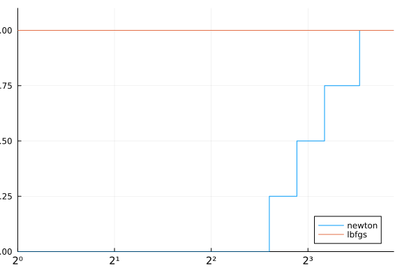
Lastly, for comparison of the methods, it is costumary to show a Performance Profile.[2] Internally we use the package BenchmarkProfiles, though using performance_profile from SolverBenchmark will actually work directly with the output of bmark_solvers.
using Plots
performance_profile(stats, df -> df.elapsed_time)
Notice how the profile indicate that all problems were solved by newton, although it is clearly not the case. That happens because our cost function for the performance profile was only the elapsed time. A better approach would be something like.
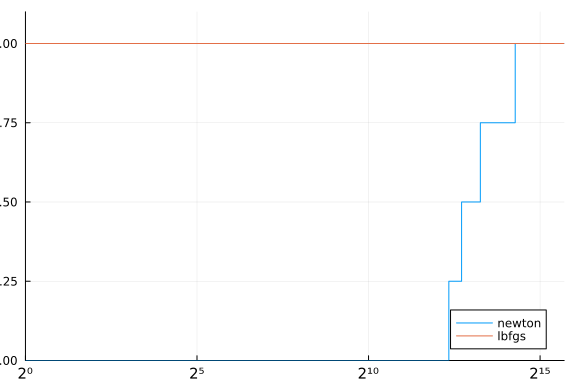
cost(df) = (df.status .!= :first_order) * Inf + df.elapsed_time
performance_profile(stats, cost)
Although we did implement the proposed method, we could improve the code a little bit. The following function is an improvement of the code in a few points:
Reuse obj(nlp, x) and grad(nlp, x) when possible.
Stopping tolerances atol and rtol are used for a stopping criteria
\[ \|\nabla f(x_k)\| \leq \epsilon_{\text{absolute}} + \epsilon_{\text{relative}}\| \nabla f(x_0)\| \]
function newton2(
  nlp :: AbstractNLPModel; # Only mandatory argument
  x :: AbstractVector = copy(nlp.meta.x0), # optimal starting point
  atol :: Real = 1e-6, # absolute tolerance
  rtol :: Real = 1e-6, # relative tolerance
  max_time :: Float64 = 30.0, # maximum allowed time
  max_iter :: Int = 100 # maximum allowed iterations
)

  # Initialization
  fx = obj(nlp, x)
  ∇fx = grad(nlp, x)

  iter = 0
  Δt = 0.0
  t₀ = time()
  α = 1e-2
  ρ = 0.0
  status = :unknown
  ϵ = atol + rtol * norm(∇fx)

  tired = Δt ≥ max_time > 0 || iter ≥ max_iter > 0
  optimal = norm(∇fx) < ϵ

  while !(optimal || tired) # while not optimal or tired

    B = Symmetric(hess(nlp, x), :L)
    factor = cholesky(B + ρ * I, check=false)
    while !issuccess(factor)
      ρ = max(1e-8, 10ρ)
      factor = cholesky(B + ρ * I, check=false)
    end
    d = factor \ -grad(nlp, x)
    ρ = ρ / 10

    t = 1.0
    ft = obj(nlp, x + t * d)
    slope = dot(grad(nlp, x), d)
    while !(ft ≤ fx + α * t * slope)
      t *= 0.5
      ft = obj(nlp, x + t * d)
    end
    t

    x += t * d

    fx = obj(nlp, x)
    ∇fx = grad(nlp, x)

    iter += 1
    Δt = time() - t₀
    tired = Δt ≥ max_time > 0 || iter ≥ max_iter > 0
    ϵ = atol + rtol * norm(∇fx)
    optimal = norm(∇fx) < ϵ
  end

  if optimal
    status = :first_order
  elseif tired
    if iter ≥ max_iter > 0
      status = :max_iter
    elseif Δt ≥ max_time > 0
      status = :max_time
    end
  end

  return GenericExecutionStats(nlp, status=status, solution=x, objective=fx, dual_feas=norm(∇fx), iter=iter, elapsed_time=Δt)

end
newton2 (generic function with 1 method)
And now testing again.
solvers = Dict(:newton => newton2, :lbfgs => lbfgs)
stats = bmark_solvers(solvers, problems)
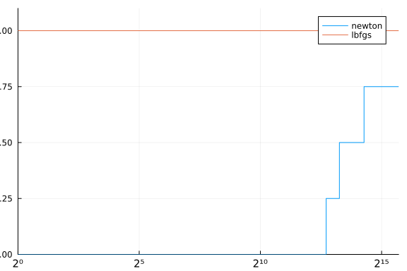
cost(df) = (df.status .!= :first_order) * Inf + df.elapsed_time
performance_profile(stats, cost)