by Tangi Migot


This package provides optimization solvers curated by the JuliaSmoothOptimizers organization. All solvers are based on NLPModels.jl and SolverCore.jl.
This package contains the implementation of four algorithms that are classical for unconstrained/bound-constrained nonlinear optimization: lbfgs, R2, tron, and trunk.
All solvers have the following signature:
stats = name_solver(nlp; kwargs...)
where name_solver can be lbfgs, R2, tron, or trunk, and with:
nlp::AbstractNLPModel{T, V} is an AbstractNLPModel or some specialization, such as an AbstractNLSModel;
stats::GenericExecutionStats{T, V} is a GenericExecutionStats, see SolverCore.jl.
The keyword arguments may include:
x::V = nlp.meta.x0: the initial guess.
atol::T = √eps(T): absolute tolerance.
rtol::T = √eps(T): relative tolerance, the algorithm stops when \(\| \nabla f(x^k) \| \leq atol + rtol \| \nabla f(x^0) \|\).
max_eval::Int = -1: maximum number of objective function evaluations.
max_time::Float64 = 30.0: maximum time limit in seconds.
verbose::Int = 0: if > 0, display iteration details every verbose iteration.
Refer to the documentation of each solver for further details on the available keyword arguments.
The solvers tron and trunk both have a specialized implementation for input models of type AbstractNLSModel.
The following examples illustrate this specialization.
using JSOSolvers, ADNLPModels
f(x) = (x[1] - 1)^2 + 4 * (x[2] - x[1]^2)^2
nlp = ADNLPModel(f, [-1.2; 1.0])
trunk(nlp, atol = 1e-6, rtol = 1e-6)
"Execution stats: first-order stationary"
nlp.counters
Counters:
             obj: ████████⋅⋅⋅⋅⋅⋅⋅⋅⋅⋅⋅⋅ 10                grad: ████████⋅⋅⋅⋅⋅⋅⋅⋅⋅⋅⋅⋅ 10                cons: ⋅⋅⋅⋅⋅⋅⋅⋅⋅⋅⋅⋅⋅⋅⋅⋅⋅⋅⋅⋅ 0
        cons_lin: ⋅⋅⋅⋅⋅⋅⋅⋅⋅⋅⋅⋅⋅⋅⋅⋅⋅⋅⋅⋅ 0             cons_nln: ⋅⋅⋅⋅⋅⋅⋅⋅⋅⋅⋅⋅⋅⋅⋅⋅⋅⋅⋅⋅ 0                 jcon: ⋅⋅⋅⋅⋅⋅⋅⋅⋅⋅⋅⋅⋅⋅⋅⋅⋅⋅⋅⋅ 0
           jgrad: ⋅⋅⋅⋅⋅⋅⋅⋅⋅⋅⋅⋅⋅⋅⋅⋅⋅⋅⋅⋅ 0                  jac: ⋅⋅⋅⋅⋅⋅⋅⋅⋅⋅⋅⋅⋅⋅⋅⋅⋅⋅⋅⋅ 0              jac_lin: ⋅⋅⋅⋅⋅⋅⋅⋅⋅⋅⋅⋅⋅⋅⋅⋅⋅⋅⋅⋅ 0
         jac_nln: ⋅⋅⋅⋅⋅⋅⋅⋅⋅⋅⋅⋅⋅⋅⋅⋅⋅⋅⋅⋅ 0                jprod: ⋅⋅⋅⋅⋅⋅⋅⋅⋅⋅⋅⋅⋅⋅⋅⋅⋅⋅⋅⋅ 0            jprod_lin: ⋅⋅⋅⋅⋅⋅⋅⋅⋅⋅⋅⋅⋅⋅⋅⋅⋅⋅⋅⋅ 0
       jprod_nln: ⋅⋅⋅⋅⋅⋅⋅⋅⋅⋅⋅⋅⋅⋅⋅⋅⋅⋅⋅⋅ 0               jtprod: ⋅⋅⋅⋅⋅⋅⋅⋅⋅⋅⋅⋅⋅⋅⋅⋅⋅⋅⋅⋅ 0           jtprod_lin: ⋅⋅⋅⋅⋅⋅⋅⋅⋅⋅⋅⋅⋅⋅⋅⋅⋅⋅⋅⋅ 0
      jtprod_nln: ⋅⋅⋅⋅⋅⋅⋅⋅⋅⋅⋅⋅⋅⋅⋅⋅⋅⋅⋅⋅ 0                 hess: ⋅⋅⋅⋅⋅⋅⋅⋅⋅⋅⋅⋅⋅⋅⋅⋅⋅⋅⋅⋅ 0                hprod: ████████████████████ 26
           jhess: ⋅⋅⋅⋅⋅⋅⋅⋅⋅⋅⋅⋅⋅⋅⋅⋅⋅⋅⋅⋅ 0               jhprod: ⋅⋅⋅⋅⋅⋅⋅⋅⋅⋅⋅⋅⋅⋅⋅⋅⋅⋅⋅⋅ 0
F(x) = [x[1] - 1; 2 * (x[2] - x[1]^2)]
nls = ADNLSModel(F, [-1.2; 1.0], 2)
trunk(nls, atol = 1e-6, rtol = 1e-6)
"Execution stats: first-order stationary"
nls.counters
Counters:
             obj: ████████⋅⋅⋅⋅⋅⋅⋅⋅⋅⋅⋅⋅ 14                grad: ██████⋅⋅⋅⋅⋅⋅⋅⋅⋅⋅⋅⋅⋅⋅ 11                cons: ⋅⋅⋅⋅⋅⋅⋅⋅⋅⋅⋅⋅⋅⋅⋅⋅⋅⋅⋅⋅ 0
        cons_lin: ⋅⋅⋅⋅⋅⋅⋅⋅⋅⋅⋅⋅⋅⋅⋅⋅⋅⋅⋅⋅ 0             cons_nln: ⋅⋅⋅⋅⋅⋅⋅⋅⋅⋅⋅⋅⋅⋅⋅⋅⋅⋅⋅⋅ 0                 jcon: ⋅⋅⋅⋅⋅⋅⋅⋅⋅⋅⋅⋅⋅⋅⋅⋅⋅⋅⋅⋅ 0
           jgrad: ⋅⋅⋅⋅⋅⋅⋅⋅⋅⋅⋅⋅⋅⋅⋅⋅⋅⋅⋅⋅ 0                  jac: ⋅⋅⋅⋅⋅⋅⋅⋅⋅⋅⋅⋅⋅⋅⋅⋅⋅⋅⋅⋅ 0              jac_lin: ⋅⋅⋅⋅⋅⋅⋅⋅⋅⋅⋅⋅⋅⋅⋅⋅⋅⋅⋅⋅ 0
         jac_nln: ⋅⋅⋅⋅⋅⋅⋅⋅⋅⋅⋅⋅⋅⋅⋅⋅⋅⋅⋅⋅ 0                jprod: ⋅⋅⋅⋅⋅⋅⋅⋅⋅⋅⋅⋅⋅⋅⋅⋅⋅⋅⋅⋅ 0            jprod_lin: ⋅⋅⋅⋅⋅⋅⋅⋅⋅⋅⋅⋅⋅⋅⋅⋅⋅⋅⋅⋅ 0
       jprod_nln: ⋅⋅⋅⋅⋅⋅⋅⋅⋅⋅⋅⋅⋅⋅⋅⋅⋅⋅⋅⋅ 0               jtprod: ⋅⋅⋅⋅⋅⋅⋅⋅⋅⋅⋅⋅⋅⋅⋅⋅⋅⋅⋅⋅ 0           jtprod_lin: ⋅⋅⋅⋅⋅⋅⋅⋅⋅⋅⋅⋅⋅⋅⋅⋅⋅⋅⋅⋅ 0
      jtprod_nln: ⋅⋅⋅⋅⋅⋅⋅⋅⋅⋅⋅⋅⋅⋅⋅⋅⋅⋅⋅⋅ 0                 hess: ⋅⋅⋅⋅⋅⋅⋅⋅⋅⋅⋅⋅⋅⋅⋅⋅⋅⋅⋅⋅ 0                hprod: ⋅⋅⋅⋅⋅⋅⋅⋅⋅⋅⋅⋅⋅⋅⋅⋅⋅⋅⋅⋅ 0
           jhess: ⋅⋅⋅⋅⋅⋅⋅⋅⋅⋅⋅⋅⋅⋅⋅⋅⋅⋅⋅⋅ 0               jhprod: ⋅⋅⋅⋅⋅⋅⋅⋅⋅⋅⋅⋅⋅⋅⋅⋅⋅⋅⋅⋅ 0             residual: ████████⋅⋅⋅⋅⋅⋅⋅⋅⋅⋅⋅⋅ 14
    jac_residual: ⋅⋅⋅⋅⋅⋅⋅⋅⋅⋅⋅⋅⋅⋅⋅⋅⋅⋅⋅⋅ 0       jprod_residual: ██████████████⋅⋅⋅⋅⋅⋅ 26     jtprod_residual: ████████████████████ 38
   hess_residual: ⋅⋅⋅⋅⋅⋅⋅⋅⋅⋅⋅⋅⋅⋅⋅⋅⋅⋅⋅⋅ 0       jhess_residual: ⋅⋅⋅⋅⋅⋅⋅⋅⋅⋅⋅⋅⋅⋅⋅⋅⋅⋅⋅⋅ 0       hprod_residual: ⋅⋅⋅⋅⋅⋅⋅⋅⋅⋅⋅⋅⋅⋅⋅⋅⋅⋅⋅⋅ 0
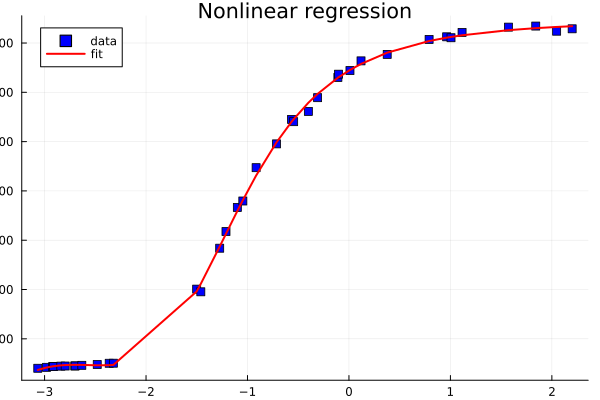
We conclude these examples by a nonlinear regression example from the NIST data set. In particular, we consider the problem Thurber.
We build a nonlinear model m with a vector of unknown parameters β.
m(β, x) = (β[1] + β[2] * x + β[3] * x^2 + β[4] * x^3) / (1 + β[5] * x + β[6] * x^2 + β[7] * x^3) # nonlinear models with unknown β vector

using CSV, DataFrames
url_prefix = "https://gist.githubusercontent.com/abelsiqueira/8ca109888b22b6ab1e76825f0567c668/raw/f3f38d61f750b443fb4307efbf853447275441a5/"
data = CSV.read(download(joinpath(url_prefix, "thurber.csv")), DataFrame)
x, y = data.x, data.y
([-3.067, -2.981, -2.921, -2.912, -2.84, -2.797, -2.702, -2.699, -2.633, -2.481  …  0.119, 0.377, 0.79, 0.963, 1.006, 1.115, 1.572, 1.841, 2.047, 2.2], [80.574, 84.248, 87.264, 87.195, 89.076, 89.608,
 89.868, 90.101, 92.405, 95.854  …  1327.543, 1353.863, 1414.509, 1425.208, 1421.384, 1442.962, 1464.35, 1468.705, 1447.894, 1457.628])
We now define the nonlinear least squares associated with the regression problem.
F(β) = [m(β, xi) - yi for (xi, yi) in zip(x, y)]
β0 = CSV.read(download(joinpath(url_prefix, "thurber-x0.csv")), DataFrame).beta
ndata = length(x)
nls = ADNLSModel(F, β0, ndata)
ADNLSModel - Nonlinear least-squares model with automatic differentiation backend ADModelBackend{
  ForwardDiffADGradient,
  ForwardDiffADHvprod,
  EmptyADbackend,
  EmptyADbackend,
  EmptyADbackend,
  ForwardDiffADHessian,
  EmptyADbackend,
}
  Problem name: Generic
   All variables: ████████████████████ 7      All constraints: ⋅⋅⋅⋅⋅⋅⋅⋅⋅⋅⋅⋅⋅⋅⋅⋅⋅⋅⋅⋅ 0        All residuals: ████████████████████ 37
            free: ████████████████████ 7                 free: ⋅⋅⋅⋅⋅⋅⋅⋅⋅⋅⋅⋅⋅⋅⋅⋅⋅⋅⋅⋅ 0               linear: ⋅⋅⋅⋅⋅⋅⋅⋅⋅⋅⋅⋅⋅⋅⋅⋅⋅⋅⋅⋅ 0
           lower: ⋅⋅⋅⋅⋅⋅⋅⋅⋅⋅⋅⋅⋅⋅⋅⋅⋅⋅⋅⋅ 0                lower: ⋅⋅⋅⋅⋅⋅⋅⋅⋅⋅⋅⋅⋅⋅⋅⋅⋅⋅⋅⋅ 0            nonlinear: ████████████████████ 37
           upper: ⋅⋅⋅⋅⋅⋅⋅⋅⋅⋅⋅⋅⋅⋅⋅⋅⋅⋅⋅⋅ 0                upper: ⋅⋅⋅⋅⋅⋅⋅⋅⋅⋅⋅⋅⋅⋅⋅⋅⋅⋅⋅⋅ 0                 nnzj: (  0.00% sparsity)   259
         low/upp: ⋅⋅⋅⋅⋅⋅⋅⋅⋅⋅⋅⋅⋅⋅⋅⋅⋅⋅⋅⋅ 0              low/upp: ⋅⋅⋅⋅⋅⋅⋅⋅⋅⋅⋅⋅⋅⋅⋅⋅⋅⋅⋅⋅ 0                 nnzh: (  0.00% sparsity)   28
           fixed: ⋅⋅⋅⋅⋅⋅⋅⋅⋅⋅⋅⋅⋅⋅⋅⋅⋅⋅⋅⋅ 0                fixed: ⋅⋅⋅⋅⋅⋅⋅⋅⋅⋅⋅⋅⋅⋅⋅⋅⋅⋅⋅⋅ 0
          infeas: ⋅⋅⋅⋅⋅⋅⋅⋅⋅⋅⋅⋅⋅⋅⋅⋅⋅⋅⋅⋅ 0               infeas: ⋅⋅⋅⋅⋅⋅⋅⋅⋅⋅⋅⋅⋅⋅⋅⋅⋅⋅⋅⋅ 0
            nnzh: (  0.00% sparsity)   28              linear: ⋅⋅⋅⋅⋅⋅⋅⋅⋅⋅⋅⋅⋅⋅⋅⋅⋅⋅⋅⋅ 0
                                                    nonlinear: ⋅⋅⋅⋅⋅⋅⋅⋅⋅⋅⋅⋅⋅⋅⋅⋅⋅⋅⋅⋅ 0
                                                         nnzj: (------% sparsity)

  Counters:
             obj: ⋅⋅⋅⋅⋅⋅⋅⋅⋅⋅⋅⋅⋅⋅⋅⋅⋅⋅⋅⋅ 0                 grad: ⋅⋅⋅⋅⋅⋅⋅⋅⋅⋅⋅⋅⋅⋅⋅⋅⋅⋅⋅⋅ 0                 cons: ⋅⋅⋅⋅⋅⋅⋅⋅⋅⋅⋅⋅⋅⋅⋅⋅⋅⋅⋅⋅ 0
        cons_lin: ⋅⋅⋅⋅⋅⋅⋅⋅⋅⋅⋅⋅⋅⋅⋅⋅⋅⋅⋅⋅ 0             cons_nln: ⋅⋅⋅⋅⋅⋅⋅⋅⋅⋅⋅⋅⋅⋅⋅⋅⋅⋅⋅⋅ 0                 jcon: ⋅⋅⋅⋅⋅⋅⋅⋅⋅⋅⋅⋅⋅⋅⋅⋅⋅⋅⋅⋅ 0
           jgrad: ⋅⋅⋅⋅⋅⋅⋅⋅⋅⋅⋅⋅⋅⋅⋅⋅⋅⋅⋅⋅ 0                  jac: ⋅⋅⋅⋅⋅⋅⋅⋅⋅⋅⋅⋅⋅⋅⋅⋅⋅⋅⋅⋅ 0              jac_lin: ⋅⋅⋅⋅⋅⋅⋅⋅⋅⋅⋅⋅⋅⋅⋅⋅⋅⋅⋅⋅ 0
         jac_nln: ⋅⋅⋅⋅⋅⋅⋅⋅⋅⋅⋅⋅⋅⋅⋅⋅⋅⋅⋅⋅ 0                jprod: ⋅⋅⋅⋅⋅⋅⋅⋅⋅⋅⋅⋅⋅⋅⋅⋅⋅⋅⋅⋅ 0            jprod_lin: ⋅⋅⋅⋅⋅⋅⋅⋅⋅⋅⋅⋅⋅⋅⋅⋅⋅⋅⋅⋅ 0
       jprod_nln: ⋅⋅⋅⋅⋅⋅⋅⋅⋅⋅⋅⋅⋅⋅⋅⋅⋅⋅⋅⋅ 0               jtprod: ⋅⋅⋅⋅⋅⋅⋅⋅⋅⋅⋅⋅⋅⋅⋅⋅⋅⋅⋅⋅ 0           jtprod_lin: ⋅⋅⋅⋅⋅⋅⋅⋅⋅⋅⋅⋅⋅⋅⋅⋅⋅⋅⋅⋅ 0
      jtprod_nln: ⋅⋅⋅⋅⋅⋅⋅⋅⋅⋅⋅⋅⋅⋅⋅⋅⋅⋅⋅⋅ 0                 hess: ⋅⋅⋅⋅⋅⋅⋅⋅⋅⋅⋅⋅⋅⋅⋅⋅⋅⋅⋅⋅ 0                hprod: ⋅⋅⋅⋅⋅⋅⋅⋅⋅⋅⋅⋅⋅⋅⋅⋅⋅⋅⋅⋅ 0
           jhess: ⋅⋅⋅⋅⋅⋅⋅⋅⋅⋅⋅⋅⋅⋅⋅⋅⋅⋅⋅⋅ 0               jhprod: ⋅⋅⋅⋅⋅⋅⋅⋅⋅⋅⋅⋅⋅⋅⋅⋅⋅⋅⋅⋅ 0             residual: ⋅⋅⋅⋅⋅⋅⋅⋅⋅⋅⋅⋅⋅⋅⋅⋅⋅⋅⋅⋅ 0
    jac_residual: ⋅⋅⋅⋅⋅⋅⋅⋅⋅⋅⋅⋅⋅⋅⋅⋅⋅⋅⋅⋅ 0       jprod_residual: ⋅⋅⋅⋅⋅⋅⋅⋅⋅⋅⋅⋅⋅⋅⋅⋅⋅⋅⋅⋅ 0      jtprod_residual: ⋅⋅⋅⋅⋅⋅⋅⋅⋅⋅⋅⋅⋅⋅⋅⋅⋅⋅⋅⋅ 0
   hess_residual: ⋅⋅⋅⋅⋅⋅⋅⋅⋅⋅⋅⋅⋅⋅⋅⋅⋅⋅⋅⋅ 0       jhess_residual: ⋅⋅⋅⋅⋅⋅⋅⋅⋅⋅⋅⋅⋅⋅⋅⋅⋅⋅⋅⋅ 0       hprod_residual: ⋅⋅⋅⋅⋅⋅⋅⋅⋅⋅⋅⋅⋅⋅⋅⋅⋅⋅⋅⋅ 0
As shown before, we can use any JSOSolvers solvers to solve this problem, but since trunk has a specialized version for unconstrained NLS, we will use it, with a time limit of 60 seconds.
stats = trunk(nls, max_time = 60.)
stats.solution
7-element Vector{Float64}:
 1288.1396826441605
 1491.255092722479
  583.3669627041016
   75.44128919391854
    0.9664368403070315
    0.39804057172490376
    0.049747755368081494
using Plots
scatter(x, y, c=:blue, m=:square, title="Nonlinear regression", lab="data")
plot!(x, t -> m(stats.solution, t), c=:red, lw=2, lab="fit")
For advanced usage, first define a Solver structure to preallocate the memory used in the algorithm, and then call solve!.
using JSOSolvers, ADNLPModels
nlp = ADNLPModel(x -> sum(x.^2), ones(3));
solver = LBFGSSolver(nlp; mem = 5);
stats = solve!(solver, nlp)
"Execution stats: first-order stationary"
The following table provides the correspondance between the solvers and the solvers structures:
It is also possible to pre-allocate the output structure stats and call solve!(solver, nlp, stats).
using JSOSolvers, ADNLPModels, SolverCore
nlp = ADNLPModel(x -> sum(x.^2), ones(3));
solver = LBFGSSolver(nlp; mem = 5);
stats = GenericExecutionStats(nlp)
solve!(solver, nlp, stats)
"Execution stats: first-order stationary"
All the solvers have a callback mechanism called at each iteration, see also the Using callbacks tutorial. The expected signature of the callback is callback(nlp, solver, stats), and its output is ignored. Changing any of the input arguments will affect the subsequent iterations. In particular, setting stats.status = :user will stop the algorithm.
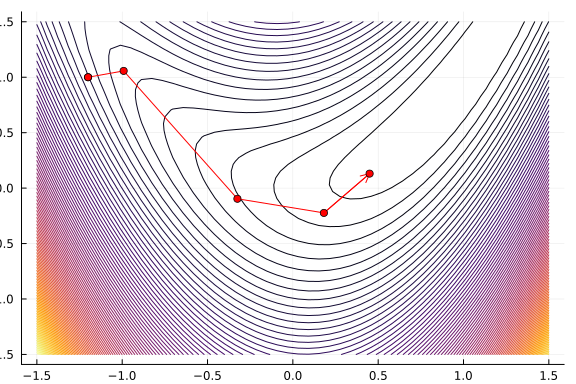
Below you can see an example of the execution of the solver trunk with a callback. It stores intermediate points until it stops the algorithm after four iterates. Afterward, we plot the iterates and create an animation from the points acquired by the callback.
using ADNLPModels, JSOSolvers, LinearAlgebra, Logging, Plots
f(x) = (x[1] - 1)^2 + 4 * (x[2] - x[1]^2)^2
nlp = ADNLPModel(f, [-1.2; 1.0])
X = [nlp.meta.x0[1]]
Y = [nlp.meta.x0[2]]
function cb(nlp, solver, stats)
  x = solver.x
  push!(X, x[1])
  push!(Y, x[2])
  if stats.iter == 4
    stats.status = :user
  end
end
stats = trunk(nlp, callback=cb)
"Execution stats: user-requested stop"
plot(leg=false)
xg = range(-1.5, 1.5, length=50)
yg = range(-1.5, 1.5, length=50)
contour!(xg, yg, (x1,x2) -> f([x1; x2]), levels=100)
plot!(X, Y, c=:red, l=:arrow, m=4)